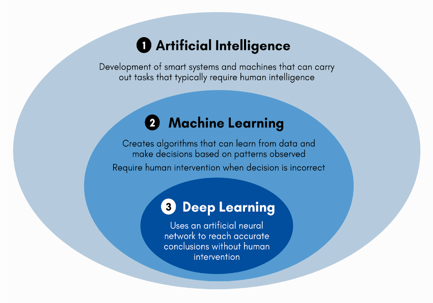
Deep learning
Deep learning, a subset of machine learning, focuses on using neural networks architecture with many layers to model complex patterns in data.
Deep learning models, often called deep neural networks, consist of multiple layers of interconnected nodes. Each layer transforms the input data into a more abstract representation, allowing the network to learn intricate patterns.
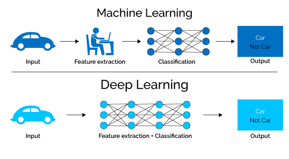
Unlike traditional machine learning, which often requires manual feature extraction, deep learning models automatically learn to extract relevant features from raw data. This capability is especially useful for tasks such as image, audio and speech recognition.
When to use deep learning?
- Complex patterns or representations
- Feature extraction is cumbersome (e.g images, audio)
Common deep learning architectures
- CNNs for image processing,
- RNNs for sequential data, and
- Transformers for NLP.
Practical Applications
Deep learning powers many modern AI applications, including self-driving cars, voice assistants, and medical image analysis, and has revolutionized the field of AI by enabling machines to perform tasks previously thought to be possible only for humans.
Inspiration
| Biological Neuron | Articficial Neuron |
|---|---|
 |
 |
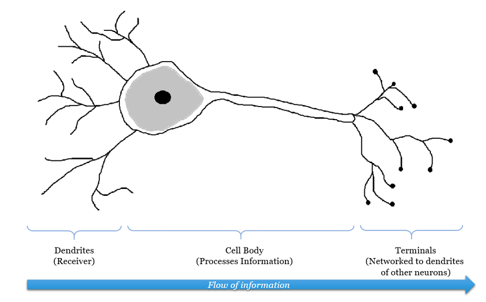
| Our brain has a large network of interlinked neurons, which acts as a highway for information to be transmitted from point A to point B. - At each neuron, its dendrites receive incoming signals sent by other neurons. - If the neuron receives a high enough level of signals within a certain period of time, the neuron sends an electrical pulse into the terminals. - These outgoing signals are then received by other neurons. |
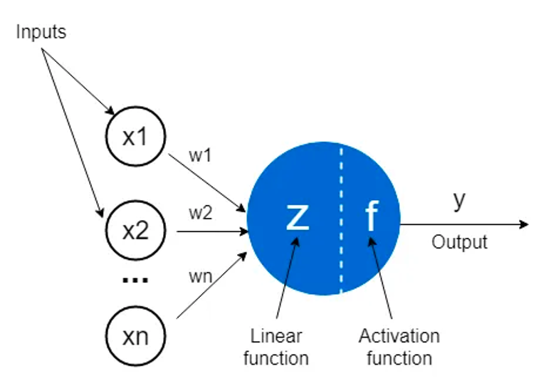
An artificial neuron is a mathematical function conceived as a model of biological neurons, a neural network . Artificial neurons are elementary units in an artificial neural network. What happens in an artificial neuron? - Multiple inputs are received - Based on individual weights associated with each input,summation occurs. - A final activation function acts on top of the summed value, generating the output. |
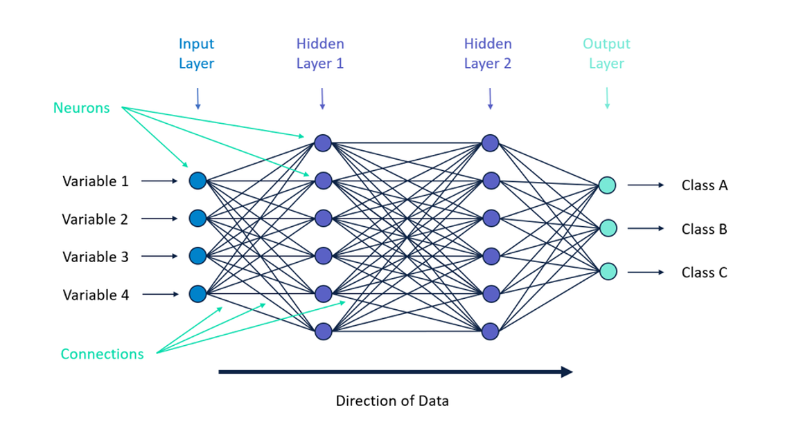
Artificial Neural Networks (ANN)
- Artificial Neural Network (ANN) is a combination of multi-layer neural network with neurons present at each layer.
- A basic ANN architecture consists of computational units and links.
- The links have different weights on themselves depending on the weightage of different connections across the network.
Multi-Layer Perceptron (MLP), Feed Forward Neural Network (FNN)
Artificial Neural Network (ANN) is a broader term that can refer to any neural network architecture, while Multi-Layer Perceptron (MLP) specifically refers to a type of ANN with a feedforward, fully connected structure.
Note The terms MLP and FNN are often used interchangeably. Technically, an FNN is any network where information flows in one direction (no cycles), while an MLP is a specific fully connected FNN with one or more hidden layers.
Core Characteristics
- The MLP falls under the category of feedforward algorithms ➛ inputs are combined with initial weights in a weighted sum and passed through an activation function. This output is fed forward to the next layer as its input, and the process continues until the output layer is reached.
- An MLP consists of:
- Input layer – receives the raw feature data
- One or more hidden layers – many neurons stacked together to learn intermediate representations
- Output layer – produces the final prediction
- Connections between nodes do NOT form cycles (i.e., no feedback loops).
- Each linear combination is propagated forward, layer by layer, from input through the hidden layers to the output layer.
- It is fully connected, meaning every neuron in one layer connects to every neuron in the next.
MLP as a Universal Function Approximator
- MLPs allow for the modeling of non-linear relationships between input and output variables, enabling them to solve tasks such as regression, classification, and pattern recognition.
- The Universal Approximation Theorem states that an MLP with at least one hidden layer and a finite number of neurons can approximate any continuous function, given appropriate weights and activation functions.
Example: An MLP can approximate sinusoidal functions, which are periodic and non-linear, by combining the outputs of neurons that each learn to approximate different parts of the sine curve.
Advantages of FNN
| Advantage | Explanation |
|---|---|
| Non-linear Modeling | By using non-linear activation functions, FNNs can capture complex relationships that linear models cannot. |
| Universal Approximation | With sufficient neurons and at least one hidden layer, they can approximate virtually any continuous function. |
| Scalability & Parallelization | Matrix-based computations are highly parallelizable, making them well-suited for GPU acceleration and large datasets. |
| End-to-End Learning | The network learns features directly from raw input to output, reducing the need for manual feature engineering. |
| Generalization | When properly trained and regularized, FNNs generalize well to unseen data. |
| Transfer Learning | Pre-trained layers/weights can be reused and fine-tuned for related tasks, saving training time and data. |
Limitations of FNN
| Limitation | Explanation |
|---|---|
| Lack of Sequential Modeling | FNNs treat inputs independently and cannot naturally capture temporal or sequential dependencies (unlike RNNs/Transformers). |
| Inefficient Parameter Sharing | Unlike CNNs, FNNs do not share weights across spatial regions, leading to a large number of parameters and higher computational cost. |
| Handling Variable-Length Inputs | They require fixed-size inputs, making them poorly suited for data of varying length (e.g., text, time series). |
| Lack of Memory | They have no internal state to "remember" previous inputs, limiting their use for tasks requiring context. |
| Interpretability | As "black-box" models, it is difficult to understand how individual weights contribute to a prediction. |
| Prone to Overfitting | With many parameters, FNNs can overfit small datasets without proper regularization (e.g., dropout, weight decay). |
| Vanishing/Exploding Gradients | Deep FNNs can suffer from gradient issues during backpropagation, slowing or destabilizing training. |
How does a neural network perform training?
1. Initialization (Starting Point)
Before training begins, the network's "weights" and "biases" are set to random numbers.
- Weights: determine the strength of the connection between different nodes (or "neurons") in the network.
- Biases shift the output to help the network fit the data better.
‼️ Because these starting numbers are random, the network's first few predictions will usually be completely wrong.
2. Forward Propagation (Making a Prediction)
- During this phase,input data is fed into the input layer of the network.
- As the data passes through the hidden layers, it is multiplied by the weights, added to the biases.$$z^{(l)} = W^{(l)},a^{(l-1)} + b^{(l)}$$
- An activation function
is applied on the above computes value to produce the layer's output. $$a^{(l)} = f!\left(z^{(l)}\right)$$ - This process continues moving forward through the network until it reaches the final layer, where the network outputs a prediction
.
3. Calculating the Loss (Measuring the Error)
At the end of each iteration, once the network's outer layer makes a prediction, it compares that prediction to the actual value (regression) or true value (classification). The mathematical tool used to measure the loss
- A high loss means the prediction was very inaccurate.
- A low loss means the prediction was close to the actual answer.
Backpropagation (backward propagation of errors) is the core algorithm used to train neural networks. It computes the gradient of the loss function with respect to every weight and bias in the network, then uses those gradients to update the parameters so the network makes better predictions.
4: Backward Propagation (Backpropagation)
This is where the network learns. The error flows backward from the output layer to the input layer.
- Using the chain rule of calculus, the network calculates the gradient of the loss with respect to every weight and bias.
- The gradient answers the question: "If I change this particular weight slightly, how much will the total error change?"
This tells the network the direction and magnitude in which each weight should be adjusted.
5. Gradient Descent (Adjusting the Weights)
Once the network knows how much each weight contributed to the error, it uses an optimization algorithm—most commonly Gradient Descent—to update the weights. $$w \leftarrow w - \eta , \nabla E$$Where:
= weight = learning rate (controls step size) = gradient of the error with respect to that weight
Weights are nudged in the opposite direction that reduces the loss.
Are ALL Weights Adjusted During Backpropagation?
| Aspect | Explanation |
|---|---|
| All weights get a gradient | Backpropagation computes a gradient for every trainable weight and bias in the network. |
| All weights are updated | During the weight-update step, all trainable parameters are adjusted simultaneously. |
| Adjustments differ in size | Each weight is adjusted by a different amount, based on how much it contributed to the error (its gradient value). |
| Some weights barely change | If a weight's gradient is very small (near zero), its update is tiny — so it changes very little. |
| Frozen layers (exception) | In transfer learning, some layers can be deliberately "frozen" so their weights are not updated, while only selected layers are trained. |
What are challenges in Backpropagation?
| Challenge | Description |
|---|---|
| Vanishing Gradients | In deep networks, gradients shrink exponentially as they propagate backward through layers with saturating activations (e.g., sigmoid, tanh), making early layers learn very slowly. Mitigated by ReLU-family activations or batch normalization. |
| Exploding Gradients | Gradients can grow exponentially instead, destabilizing training. Addressed with gradient clipping or careful weight initialization. |
| High-Dimensional Loss Surface | With millions of parameters the loss landscape is highly non-convex with saddle points and local minima, making finding the global minimum challenging. |
| Computational & Memory Cost | Storing all activations from the forward pass for use in the backward pass is memory-intensive for very deep networks. |
| Sensitivity to Initialization | Poor weight initialization can lead to dead neurons or slow convergence; strategies like Xavier/He initialization help. |
How do we compare predictions to ground truth?
Loss Functions: A loss function
| Loss Function | Use Case | Formula |
|---|---|---|
| Mean Squared Error (MSE) | Regression | |
| Binary Cross-Entropy | Binary classification | |
| Categorical Cross-Entropy | Multi-class classification | |
| Huber Loss | Regression (robust to outliers) | Quadratic for small errors, linear for large |
How many times do we iterate this process?
1. "One pass through all samples = 1 epoch"
In machine learning, your dataset is made up of individual
- 1 Epoch = The network has seen the entire dataset exactly once.
2. "Multiple Epochs"
As we covered in the backpropagation steps, a neural network learns by taking tiny steps down the error gradient (controlled by the Learning Rate —
3. "Until loss converges"
This is the ultimate goal of training. Loss is the measurement of how wrong the network's predictions are.
- In the first few epochs, the network learns the most obvious patterns, and the loss drops rapidly.
- As the epochs continue, the network fine-tunes its knowledge, and the loss drops more slowly.
- Convergence happens when the loss stops decreasing and levels out into a flat horizontal line. When the loss converges, it means the network has learned everything it possibly can from that dataset, and running more epochs won't make it any smarter (and might actually cause it to memorize the data too rigidly, a problem known as "overfitting").
This is where you stop, either when the number of epoch iterations are done or when the loss stops decreasing and levels out into a flat horizontal line, whichever comes first.
What is difference between NN and ML?
| Feature | Traditional Machine Learning | Neural Networks (Deep Learning) |
|---|---|---|
| Input Data ⭐ | Requires clean, structured, tabular data. | Unstructured data (images, text, audio), highly complex problems. |
| Feature Engineering ⭐ | Manual (done by the human programmer). | Automatic (done by the network's hidden layers). |
| Model Structure | Statistical equations, decision trees. | Interconnected layers of artificial neurons. |
| Hardware | Can usually run on standard computer processors (CPUs). | Often requires specialized, powerful hardware like GPUs. |
| Training Time | Generally fast to train (minutes to hours). | Can be extremely slow to train (days to weeks). |
| Interpretability | High ("White Box"). It is easy to track how the math led to the result. | Low ("Black Box"). It is very difficult to explain exactly how it reached its specific conclusion. |
| Scalability | Plateaus in performance after a certain amount of data. | Continues to improve as you feed it more data. |